
If you have a dataset you'd like to break into chunks and fit a model for each chunk, and you don't want to copy pasta the same code over and over, or use a clunky for loop, read on. You can do it in less than 10 lines of code using purrr::map.
Header photo by Tara Evans on Unsplash. Full code on Github.
Getting Some Data
Let's begin by generating some data using the ravelRy package (shameless self-plug), which makes knitting and crochet patterns available via Ravelry.com's API. You can follow the steps here for installing the package, creating a Ravelry developer account, and authenticating via the package.
To create a dataset, let's pass four different search terms to the ravelRy::search_patterns function using purrr:map: scarf, hat, sweater, and blanket. For each, let's restrict to crochet patterns, sort by popularity, and retrieve the top 200. The returned ids can then be used to get pattern details using the function ravelRy::get_patterns.
queries <- data.frame(query = c('scarf', 'hat', 'sweater', 'blanket')) %>%
  mutate(results = map(query, ~ search_patterns(query     = .,
                                                craft     = 'crochet',
                                                page_size = 200,
                                                sort      = 'popularity')))

ids <- queries %>%
  unnest(results)

pattern_details <- get_patterns(ids = ids$id)

patterns <- ids %>%
  select(query, id) %>%
  left_join(pattern_details, by = 'id') %>%
  mutate(yardage = as.numeric(yardage)) %>%
  filter(!is.na(yardage), !is.na(difficulty_average))
Looking at The Data
The relationship of interest here is the impact of pattern yardage on the average pattern difficulty score. Are bigger projects also more challenging?
yardage_boxplot <- patterns %>%
  ggplot(aes(x = yardage, y = query)) +
  geom_boxplot() +
  labs(title = 'Yardage by search term')

difficulty_boxplot <- patterns %>%
  ggplot(aes(x = difficulty_average, y = query)) +
  geom_boxplot() +
  labs(title = 'Average difficulty by search term')

yardage_difficulty_scatter <- patterns %>%
  ggplot(aes(x = yardage, y = difficulty_average, color = query)) +
  geom_point() +
  facet_wrap(~query) +
  labs(title = 'Difficulty and yardage by search term') +
  theme(legend.position = 'none')

gridExtra::grid.arrange(yardage_boxplot, difficulty_boxplot, yardage_difficulty_scatter,
                        padding = unit(0.15, "line"),
                        heights = c(2,3),
                        layout_matrix = rbind(c(1,2), c(3)))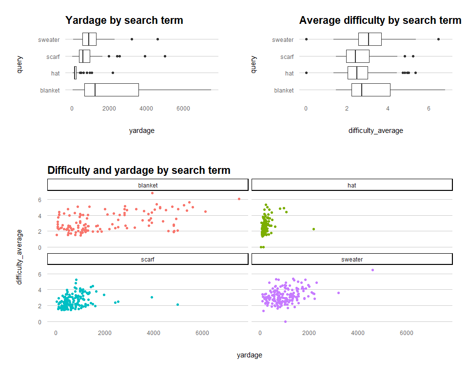
There are various other data cleansing (such as outlier removal, looking at those scatter plots) and transformation steps that should be considered here, but for the sake of demonstrating how to fit the models, we'll breeze past those.
Nesting the Data and Fitting the Models
Next, we can nest the data under each query, split into training and testing subsets, fit the a linear regression model, and calculate predictions using map.
set.seed(1234)
nested_fit <- patterns %>%
  select(query, id, yardage, difficulty_average) %>%
  nest(-query) %>%
  mutate(split = map(data, ~initial_split(., prop = 8/10)),
         train = map(split, ~training(.)),
         test  = map(split, ~testing(.)),
         fit   = map(train, ~lm(difficulty_average ~ yardage, data = .)),
         pred  = map2(.x = fit, .y = test, ~predict(object = .x, newdata = .y)))
There is a lot to unpack here! First, I reduced the data down to just the columns of interest, and then nested them within the query value. You could also think about this as creating a single row for each of the four query values and sticking all the according data into a list-column called data. From there, you can manipulate that list-column using map.
Next, I split each query's data into 80% training, 20% testing using; created the training and testing data; and fit the linear model using lm. Each step uses map to pass a list-column into a function. Finally, I used map2 to pass 2 list-columns into the predict function. You end up with a tibble that looks like this:
|
query <chr> |
data <list> |
split <list> |
train <list> |
test <list> |
fit <list> |
pred <list> |
|---|---|---|---|---|---|---|
| scarf | <tibble> | <S3: rsplit> | <tibble> | <tibble> | <S3: lm> | <dbl [34]> |
| hat | <tibble> | <S3: rsplit> | <tibble> | <tibble> | <S3: lm> | <dbl [34]> |
| sweater | <tibble> | <S3: rsplit> | <tibble> | <tibble> | <S3: lm> | <dbl [34]> |
| blanket | <tibble> | <S3: rsplit> | <tibble> | <tibble> | <S3: lm> | <dbl [34]> |
To view the fit for each model, the function broom::glance can be mapped to each fit and unnested.
nested_fit %>%
  mutate(glanced = map(fit, glance)) %>%
  select(query, glanced) %>%
  unnest(glanced)


## # A tibble: 4 x 13
##   query r.squared adj.r.squared sigma statistic p.value    df logLik  AIC
##   <chr>     <dbl>         <dbl> <dbl>     <dbl>   <dbl> <dbl>  <dbl> <dbl>
## 1 scarf    0.0496        0.0421 0.777      6.68 1.09e-2     1  -151.  307.
## 2 hat      0.0770        0.0680 0.881      8.51 4.35e-3     1  -133.  273.
## 3 swea~    0.172         0.165  0.821     28.2  4.43e-7     1  -168.  341.
## 4 blan~    0.184         0.176  1.09      21.9  9.45e-6     1  -148.  303.
## # ... with 4 more variables: BIC <dbl>, deviance <dbl>, df.residual <int>, nobs <int>
The adj.r.squared values are quite low, but we do have a small dataset. Next let's inspect the coefficients.
nested_fit %>%
  mutate(tidied = map(fit, tidy)) %>%
  select(query, tidied) %>%
  unnest(tidied)


## # A tibble: 8 x 6
##   query   term        estimate std.error statistic  p.value
##   <chr>   <chr>          <dbl>     <dbl>     <dbl>    <dbl>
## 1 scarf   (Intercept) 2.23     0.117         19.0  6.78e-39
## 2 scarf   yardage     0.000510 0.000134       3.81 2.14e- 4
## 3 hat     (Intercept) 2.01     0.128         15.7  8.27e-29
## 4 hat     yardage     0.00299  0.000514       5.81 7.30e- 8
## 5 sweater (Intercept) 2.66     0.128         20.7  6.24e-44
## 6 sweater yardage     0.000578 0.000109       5.31 4.43e- 7
## 7 blanket (Intercept) 2.56     0.176         14.6  3.71e-26
## 8 blanket yardage     0.000295 0.0000630      4.68 9.45e- 6
Test Set Prediction
Despite low R2 for the models, the coefficients are all significant. How good are they at predicting the test set values?
nested_fit_evaluate <- nested_fit %>%
  select(query, test, pred) %>%
  unnest(test, pred)

nested_fit_evaluate %>%
  group_by(query) %>%
  summarise(total_ss = sum((difficulty_average - mean(difficulty_average))^2),
            residual_ss = sum((difficulty_average - pred)^2),
            n = n(),
            .groups = 'drop') %>%
  mutate(r.squared = 1 - (residual_ss/total_ss),
         adj.r.squared = 1 - (((1-r.squared)*(n-1))/(n-1-1)))


## # A tibble: 4 x 6
##   query   total_ss residual_ss     n r.squared adj.r.squared
##   <chr>      <dbl>       <dbl> <int>     <dbl>         <dbl>
## 1 blanket     29.6        18.8    24    0.365        0.336
## 2 hat         17.3        12.3    25    0.289        0.259
## 3 scarf       16.1        13.9    32    0.132        0.103
## 4 sweater     30.0        29.1    34    0.0290      -0.00135
The blanket, hat and scarf models do a pretty good job of predicting the test set values, but sweater is poor.
Why not just fit one big model?
How does nested data linear models compare to one large model where the nesting value is a categorical independent variable? Guess what. It's the same!
set.seed(2345)
split <- initial_split(patterns, prop = 8/10, strata = query)
pattern_train <- training(split)
pattern_test <- testing(split)

fit <- lm(difficulty_average ~ yardage*query, data = pattern_train)

fit %>%
  tidy()


## # A tibble: 8 x 5
##   term                   estimate std.error statistic  p.value
##   <chr>                     <dbl>     <dbl>     <dbl>    <dbl>
## 1 (Intercept)           2.42      0.135        17.9   5.87e-55
## 2 yardage               0.000340  0.0000499     6.80  3.21e-11
## 3 queryhat             -0.0481    0.177        -0.272 7.86e- 1
## 4 queryscarf           -0.0484    0.180        -0.269 7.88e- 1
## 5 querysweater          0.163     0.192         0.849 3.97e- 1
## 6 yardage:queryhat      0.000750  0.000340      2.21  2.79e- 2
## 7 yardage:queryscarf   -0.0000650 0.000132     -0.493 6.22e- 1
## 8 yardage:querysweater  0.000261  0.000127      2.05  4.06e- 2
In the single model, the formula is Y = B0 + B1X1 + B2X2 + B3X1X2 + error,
- where Y is
difficulty_average, X1 isyardage, X2 isquery - B0 is the intercept, B1 is the coefficient for yardage, B2 is the coefficient for query, and B3 is the coefficient for the interaction term
The big ugly formula would be:
Y =
2.42 +
0.000340* yardage +
-0.0481* query(hat) +
-0.0484* query(scarf) +
0.163* query(sweater) +
0.000750* yardage * query(hat) +
-0.000065* yardage * query(scarf) +
0.000261* yardage * query(sweater) +
error
Where query(hat) is 1 when query = "hat" and 0 otherwise. So for hat, we could replace both query(hat) with 1s, and the other query(x) to zeroes and simplify to:
Y = 2.42 + 0.000340* yardage + -0.0481 + 0.000750* yardage
And then move terms: Y = (2.42 -0.0481) + (0.000340 + 0.000750)* yardage
Finally: Y = 2.376 + 0.00109006* yardage
Basically, the summarized coefficients for each query is the addition of the intercept and query term, and the addition of the yardage and interaction term. We get the same results if we run 4 models on the nested data:
nested_fit_test <- pattern_train %>%
  select(query, id, yardage, difficulty_average) %>%
  nest(-query) %>%
  mutate(fit = map(data, ~lm(difficulty_average ~ yardage, data = .)))

nested_fit_test %>%
  mutate(tidied = map(fit, tidy)) %>%
  select(query, tidied) %>%
  unnest(tidied)

## # A tibble: 8 x 6
##   query   term        estimate std.error statistic  p.value
##   <chr>   <chr>          <dbl>     <dbl>     <dbl>    <dbl>
## 1 scarf   (Intercept) 2.38     0.105         22.7  1.07e-46
## 2 scarf   yardage     0.000275 0.000107       2.56 1.17e- 2
## 3 hat     (Intercept) 2.38     0.116         20.6  4.45e-38
## 4 hat     yardage     0.00109  0.000341       3.20 1.85e- 3
## 5 sweater (Intercept) 2.59     0.124         20.8  4.71e-44
## 6 sweater yardage     0.000600 0.000107       5.61 1.07e- 7
## 7 blanket (Intercept) 2.42     0.165         14.7  2.39e-26
## 8 blanket yardage     0.000340 0.0000610      5.56 2.34e- 7
So, it's really up to you whether you choose to split your data by some factor and fit multiple models or simply introduce that factor as an interaction term. If you're looking to compare a particular coefficient across factor levels, splitting and fitting multiple may be faster than extracting the terms from a large model.