Craft beer is a huge market. Beer reviews from fellow beer drinkers help customers navigate it.
From 2013 to 2016, the craft beer industry nearly doubled in value from $14.3 to $23.5 billion. The number of craft breweries jumped from 2,768 to 5,005, and production ramped up from 15 to 25 million barrels a year.
BeerAdvocate was founded in 1996 as a forum to review, rate and share ideas about beer. Today, the site houses millions of reviews for hundreds of thousands of beers, both domestic and international.
Users can rate beers and optionally provide text explaining their assessment. BeerAdvocate takes a thorough approach to beer evaluation, asking users to rate each on several features: look, smell, taste, feel, and overall. The platform also provides measures to indicate the spread or consensus of reviews, both in the rDev (a single rating's deviation from the overall mean rating) and the pDev (deviation within a beer's ratings).
There are far too many beers and breweries to conduct any kind of broad analysis at that level - so the focus will be on beer styles, of which BeerAdvocate lists about 100.
Data
A sample of beer reviews were collected from BeerAdvocate.com, resulting in a dataset of 31,550 beers and their brewery, beer style, ABV, total numerical ratings, number of text reviews, and a sample of review text. Review text was gathered only for beers with at least 5 text reviews. A minimum of 2000 characters of review text were collected for those beers, with total length ranging from 2000 to 5000 characters.
You can view the R scripts here.
What are the most characteristic words for each style?
Are IPAs defined by the word "hoppy" or stouts by "coffee"?
Do reviewers talk about double IPAs differently than regular IPAs?
Term Frequency-Inverse Document Frequency, or TF-IDF, is a statistic often used to identify keywords for document retrieval by search engines and in recommender systems to suggest similar items. It looks for terms that are frequent in a particular document but rare in other documents.
# tidy the text,
# grouping by beer style
beer_tidy <- beer_reviews %>%
  unnest_tokens(word, Review_Text) %>%
  anti_join(stop_words) %>%
  count(word, Style)

# remove beer names, calculate
# word total and tf-idf
beer_tidy_tfidf <- beer_tidy %>%
  filter(!word %in% beer_names) %>% # not included here
  group_by(word) %>%
  mutate(word_total = sum(n)) %>%
  bind_tf_idf(word, Style, n)  %>%
  subset(tf_idf > 0) %>%
  arrange(desc(tf_idf))

# create a df for plotting of
# the top 16 beers by review count
top_beers <- aggregate(Reviews ~ Style, beer_reviews, sum) %>% top_n(16, Reviews)
beer_tidy_tfidf_10 <- beer_tidy_tfidf %>%
  subset(Style %in% top_beers$Style & word_total >= 10) %>%
  group_by(Style) %>%
  top_n(10, tf_idf) %>%
  arrange(Style, desc(tf_idf)) %>%
  ungroup() %>%
  mutate(Rank = rep(10:1, 16))

# styling omitted for brevity
ggplot(beer_tidy_tfidf_10, aes(x=as.factor(Rank), y=tf_idf)) +
  geom_bar(stat="identity", fill="cadetblue", alpha=0.5) +
  coord_flip() + facet_wrap(~ Style,ncol=4) +
  geom_text(aes(label=word, x=Rank), y=0,hjust=0) +
  labs(title="Top TF-IDF Terms for Selected Beer Styles\n",
  x="", y="tf-idf")
A sample of top TF-IDF terms are displayed below for the top 16 beer styles by number of profiles.
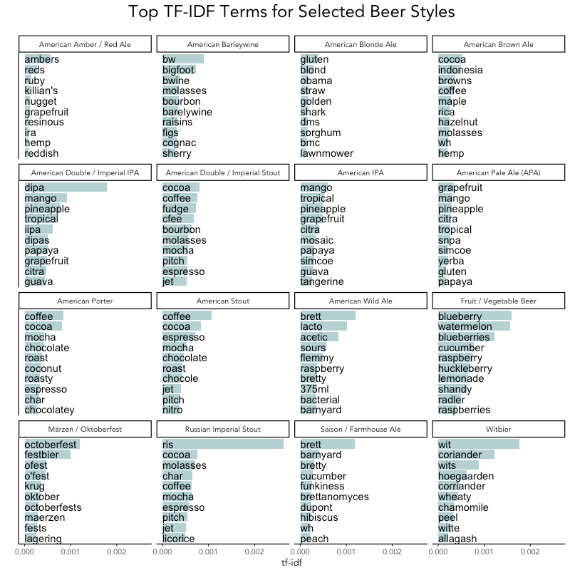
The names and styles of the beers were excluded (e.g. "American Stout") but many abbreviations rose to the top as important words (like RIS, DIPA).
Which beers are similar to each other?
Similarity between beers can often be inferred through name or origin: an imperial stout is probably similar to an American stout.
Beyond brewing style or ingredient list, can the quantified review text be used to see underlying patterns and groups within beer styles? Does the way reviewers talk about beer styles match up with their pre-defined links?
Looking at the TF-IDF results above, there's clearly overlap in important keywords between several groups. "Mango" is top word for American Double / Imperial IPA as well as American IPA and American Pale Ale. "Coffee" rises to the top for American Porter, American Stout, American Double / Imperial Stout and Russian Imperial Stout. "Raspberry" links Fruit / Vegetable Beer with American Wild Ale.
A correlation plot, with styles grouped by hierarchical clusters, shows distinct patterns in the data. This plot reveals the extent to which each beer style's review words (proportions) are similar. Darker boxes indicate higher correlation between two beer styles.
# get the proportion of words in each
# style and create a matrix with
# styles as columns and words as rows
beer_corr <- beer_tidy %>%
  subset(!is.na(Style)) %>%
  group_by(Style) %>%
  mutate(Prop = n / sum(n))  %>%
  subset(n >= 5) %>%
  select(-n) %>%
  spread(Style, Prop)

# replace NAs with 0 because an NA
# is an observation of 0 words
beer_corr[is.na(beer_corr)] <- 0

mycol <- colorRampPalette(c("darkgrey", "grey", "white", "cadetblue1", "cadetblue"))
corr <- cor(beer_corr[,-1], use = "pairwise.complete.obs") %>%
  corrplot(method="color", order="hclust", diag=FALSE,
           tl.col = "black", tl.srt = 45, tl.cex=0.6,
           col=mycol(100),
           type="lower",
           title="Correlation Between Beer Styles",
           family="Avenir",
           mar=c(0,0,1,0))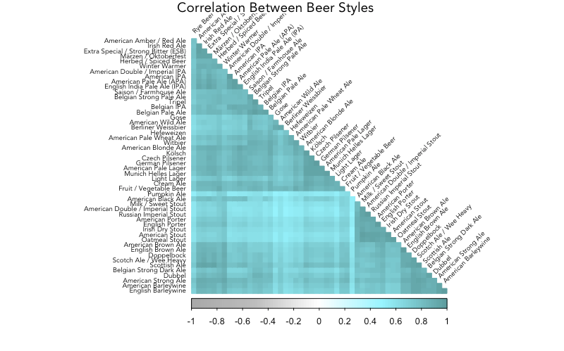
It's easy to spot similar groups with stouts and porters clustered together, IPAs and APAs grouped, and Belgian beers in close proximity. Pumpkin Ale is an outlier, with its dissimilarity from all other beers a clear light-colored line.
Hierarchical clustering is a method that begins by treating each group distinctly and then merges the closest groups together repeatedly until all have combined. It produces a dendrogram, or tree plot, that makes visualizing the distance (Euclidean, in this instance) between groups easy.
# transpose the matrix to have styles
# as rows and words as columns
beer_corr_t <- t(beer_corr[,-1])

# calculate distance
beer_dist <- dist(beer_corr_t, method="euclidean")

# fit clusters
fit <- hclust(beer_dist, method="ward.D")

# plot
plot(fit,main="Cluster Dendrogram of Beer Styles",
    family="Avenir")
rect.hclust(fit, k=8, border="cadetblue")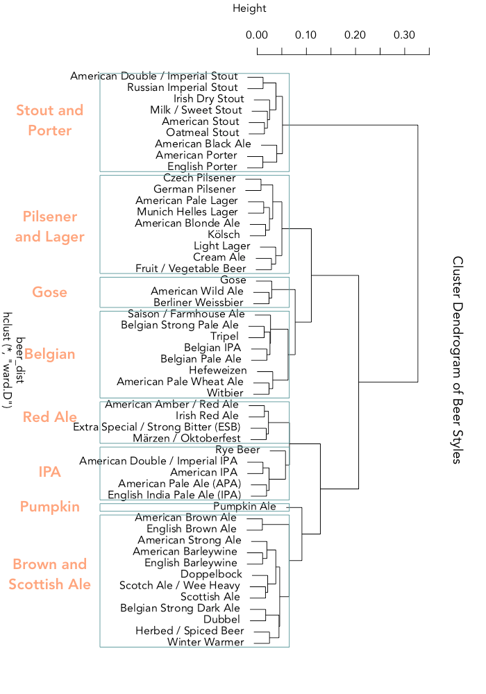
Eight clusters were chosen for ease of interpretability (diagnostics that help determine the number of clusters gave no concrete figure). I rotated the plot and added the labels afterward.
The way reviewers talk about stouts and porters is so different from other beers that they have their own branch, which further splits to separate stouts from the porters and black ale.
Pumpkin ale is reviewed so differently from others that it's the only beer style to have a cluster all to itself (though it looks like rye beer came close).
Can we predict a beer's style by its review?
Given reviews for a new beer, can we accurately guess what type of beer it is?
k-Nearest Neighbors (kNN) is an algorithm used to classify observations into predetermined groups.
Using kNN on a small subset (20%) of the dataset, accuracy ranged from 58% to 93%, depending on the cluster. Stouts and porters and IPAs were the most accurate in classification, while beers in the Gose cluster were often confused with beers from the Belgian cluster.
# add groups to the dataset
groupnames <- data.frame(
  Name=c("Red Ale", "Brown and Scottish Ale", "Stout and Porter",
     "Pilsener and Lager", "IPA", "Belgian", "Gose", "Pumpkin"),
     Group=c(1:8))
groups <- data.frame(cutree(fit, k=8)) %>%
  set_colnames("Group") %>%
  mutate(Style = row.names(.)) %>%
  left_join(groupnames, "Group")
beer_kgroup <- merge(beer_reviews[beer_reviews$Style %in% groups$Style
     & !is.na(beer_reviews$Review_Text),],
     groups[,2:3], by="Style", all=T)

# tidy the text by individual beer review, keeping words
# that account for at least 0.05% of a review
beer_corr_knn <- beer_kgroup %>%
  unnest_tokens(word, Review_Text) %>%
  anti_join(stop_words) %>%
  count(word, Beer_URL) %>%
  group_by(Beer_URL) %>%
  mutate(Prop = n / sum(n))  %>%
  subset(Prop >= .005) %>%
  select(-n) %>%
  spread(word, Prop) %>%
  left_join(beer_kgroup[,c(2,13)], by = "Beer_URL")
beer_corr_knn[is.na(beer_corr_knn)] <- 0

# randomly take 20% of the dataset
set.seed(1234)
subset_ids <- sample(1:length(beer_corr_knn$Beer_URL), length(beer_corr_knn$Beer_URL)*.20, replace=F)
beer_corr_subset <- beer_corr_knn[subset_ids, ]

# split that into 80% training and 20% test
train_ids <- sample(length(beer_corr_subset$Beer_URL), length(beer_corr_subset$Beer_URL)*.80, replace=F)
last <- length(beer_corr_predict)
train_bk <- beer_corr_subset[train_ids, -c(1,last)] # training
test_bk <- beer_corr_subset[-train_ids, -c(1,last)] # testing
train_resp <- beer_corr_subset[train_ids, c(1,last)] # groups for training
test_resp <- beer_corr_subset[-train_ids, c(1,last)] # groups for testing

# run kNN
system.time(kresult <- knn(train = train_bk,
     test = test_bk,
     cl = train_resp$Name.y,
     k = 1))
# took about 10 min. to process

# check results
knn_results <- data.frame(round(prop.table(table(kresult, test_resp$GroupNum),2),2)) %>%
  set_colnames(c("Classification", "Actual", "Pct")) %>%
  mutate(Classfication = factor(Classification, labels=groupnames$Name),
         Actual = factor(Actual, labels=groupnames$Name))

# plot
ggplot(knn_results, aes(Actual, Pct, fill=Classification)) +
  geom_bar(stat="identity", position="dodge", alpha=0.75) +
  labs(title="Accuracy of KNN Classification into HClusters\n", y = "Percent") +
  theme_classic(base_size=10, base_family="Avenir") +
  theme(axis.text.x=element_text(angle=30, hjust=1)) + ylim(c(0,1))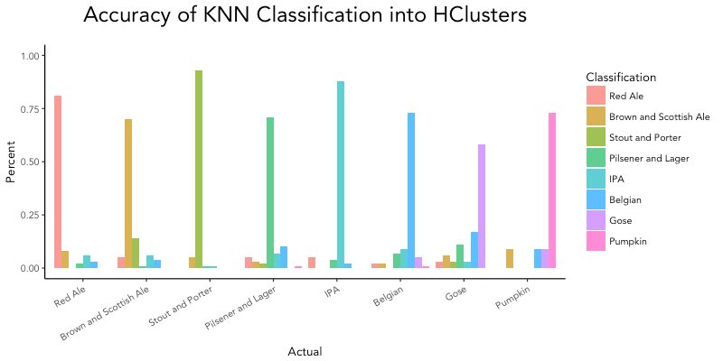
This could probably be improved by doing some dimension reduction to reduce the run time.
Summary
Beer reviews contain important and distinctive information that can be used to identify new patterns and connections between beer styles as well as underscore relationships defined by origin or brewing style.
View the R scripts here.