
How do you quantify the style progression of a band over time?
Over 20 years, several albums, the addition of Travis Barker and the exit of Tom DeLonge, blink-182's style has evolved as well as solidified.
"The band was already heading in an artier direction on 2003’s Blink-182, and drummer Travis Barker nearly died in a 2008 plane crash. So maybe it’s remarkable that the old Blink bounce – double-time tempos, crisp tuneage, self-deprecating lyrics – is intact at all." – Rolling Stone review of blink-182's 2011 album Neighborhoods
Based on the audio track features provided by the Spotify Web API, I measured the similarity between blink-182 songs and albums.
I downloaded the song data using spotifyr, found the Euclidean distance between songs using dist, clustered the songs together using hclust, and finally, visualized the results using dendextend.

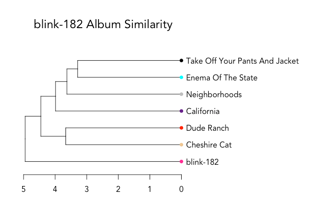
Albums are color-coded, and even with a quick look, it's clear that Cheshire Cat (1995) and Dude Ranch (1997) are close in similarity, with nearly all of their songs appearing together in the bottom half of the dendrogram. It makes sense, since the albums were consecutive, and featured the same band members (Hoppus, DeLonge, and drummer Scott Raynor).
Enema of the State (1999) and Take Off Your Pants and Jacket (2001) are also closely intertwined in the top half of the dendrogram. The albums came out closely together and initiated the band's breakthrough, as well as featured the same band members (Hoppus, DeLonge, and drummer Travis Barker). The only song to jump to the bottom of the dendrogram with the band's early work is "Happy Holidays, You Bastard."
blink-182 (2003) had a more experimental, more serious feel than the band's previous work. According to Spotify's audio features, blink-182 was more like Cheshire Cat and Dude Ranch than the albums released right before it.
In 2005, Tom DeLonge left to pursue other projects, leading the band to take a hiatus until they reunited in 2009 to produce Neighborhoods (2011). The reunion didn't last, and the band ultimately filled Tom DeLonge's place with guitarist Matt Skiva in 2015. In 2016, they released California.
The tracks from California and Neighborhoods have more in common with the band's later work - Enema of the State and Take Off Your Pants And Jacket - than the albums released before the addition of Travis Barker.
An overall look at album similarity (based on the median distance between songs in each album) tells a similar story, though blink-182 is isolated in its own branch. This is likely because several of its tracks are very different than the rest - such as "Stockholm Syndrome Interlude."
R code and explanation below as well as Github.
Background
Spotify's music library contains 40 million songs available for streaming to more than 190 million users around the world. It's all accessible via the Spotify Web API - made easier with the spotifyr API wrapper for R.
The API provides descriptive data for artists, tracks and albums, in addition to quantitative track audio features, which include measures like danceability, acousticness, liveness, energy, valence, and speechiness.
For example, Spotify defines danceability as:
Danceability describes how suitable a track is for dancing based on a combination of musical elements including tempo, rhythm stability, beat strength, and overall regularity. A value of 0.0 is least danceable and 1.0 is most danceable.
With individual songs described by a series of numeric features, there is an opportunity to identify similar and dissimilar tracks, albums, and artists by measuring the distance between them.
Method
1. Build and preprocess the dataset
Use a loop to query tracks for the three bands in question.
library(spotifyr)

Sys.setenv(SPOTIFY_CLIENT_ID = 'your_id')
Sys.setenv(SPOTIFY_CLIENT_SECRET = 'your_secret')
access_token <- get_spotify_access_token()

b_songs <- get_artist_audio_features("blink-182")
Next, filter out any extraneous albums and EPs, then reduce the dataset to the pertinent numeric features, convert the one character feature to a number, and add a location key for later use.
albums_to_compare <- c('Cheshire Cat',
  'Dude Ranch',
  'Enema Of The State',
  'Take Off Your Pants And Jacket',
  'blink-182',
  'Neighborhoods',
  'California')

b_songs2 <- b_songs %>%
  filter(album_name %in% albums_to_compare) %>%
  select(c("danceability",
    "energy",
    "loudness",
    "speechiness",
    "acousticness",
    "instrumentalness",
    "liveness",
    "valence",
    "tempo",
    "duration_ms",
    "key_mode",
    "track_popularity",
    "album_popularity",
    "artist_name",
    "track_name",
    "album_name")) %>%
  mutate(location = 1:n(),
         key_mode = as.numeric(as.factor(key_mode)))
That yields this dataframe:
str(b_songs)
Classes ‘tbl_df’, ‘tbl’ and 'data.frame':	98 obs. of  17 variables:
 $ danceability    : num  0.411 0.317 0.423 0.633 ...
 $ energy          : num  0.962 0.963 0.714 0.748 ...
 $ loudness        : num  -5.95 -6.17 -8.29 -7.78 ...
 $ speechiness     : num  0.0917 0.08 0.045 0.0594  ...
 $ acousticness    : num  0.103 0.000168 0.00113 ...
 $ instrumentalness: num  0.00 0.00 6.28e-06 3.57e-05 ...
 $ liveness        : num  0.529 0.19 0.0855 0.44 0.14 ...
 $ valence         : num  0.622 0.46 0.593 0.431 0.198 ...
 $ tempo           : num  173 170 110 119 117 ...
 $ duration_ms     : num  172646 163508 227250 219540  ...
 $ key_mode        : num  9 9 2 2 15 4 2 3 4 7 ...
 $ track_popularity: int  64 50 73 51 44 ...
 $ album_popularity: int  73 73 73 73 73 ...
 $ artist_name     : chr  "blink-182" "blink-182" ...
 $ track_name      : chr  "Feeling This" "Obvious" ...
 $ album_name      : chr  "blink-182" "blink-182" ...
 $ location        : int  1 2 3 4 5 6 7 8 9 10 ...
2. Calculate the Euclidean distance
b_dist <- b_songs %>%
  select(-c("artist_name", "track_name", "album_name", "location")) %>%
  as.matrix() %>%
  scale(center = TRUE, scale = TRUE) %>% # scale
  dist(method = "euclidean")

b_hclust <- hclust(b_dist, method = 'average')
3. Visualize the distance
dend <- b_hclust %>% as.dendrogram()

# assign a color to each album
my_colors <- b_songs$album_name %>%
  recode('California' = 'darkorchid4', 'Neighborhoods' = 'grey',
         'blink-182' = 'deeppink','Cheshire Cat' = 'burlywood2','Dude Ranch' = 'red',
         'Enema Of The State'= 'cyan1', 'Take Off Your Pants And Jacket' = 'black')
my_colors <- my_colors[order.dendrogram(dend)]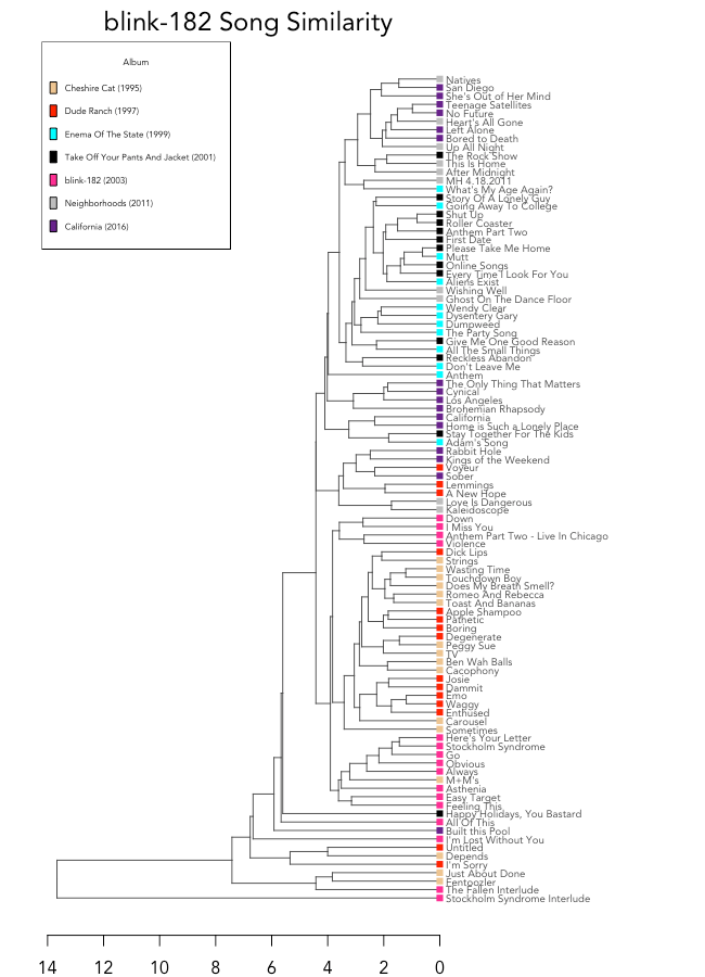
Let's summarize the distance between albums by finding the median distance between each pair.
b_album_avg <- b_dist %>%
  as.matrix() %>%
  as.data.frame() %>%
  # add in the album names for the rows
  mutate(album_name = b_songs$album_name) %>%
  # melt into a long DF
  reshape2::melt(id = 'album_name') %>%
  # add in the album names for the columns
  mutate(variable = as.numeric(as.character(variable))) %>%
  left_join(b_songs[,c('location', 'album_name')], by = c('variable' = 'location')) %>%
  # group by album pair and get the median distance
  group_by(album_name.x, album_name.y) %>%
  summarise(distance = median(value)) %>%
  # put back into a matrix format instead of a long DF
  reshape2::dcast(album_name.x ~ album_name.y, value.var = 'distance')

# return this to a dist object and cluster it
dend_album <- b_album_avg %>%
  select(-album_name.x) %>%
  as.dist() %>%
  hclust(method = 'average') %>%
  as.dendrogram()
And plot it.
par(mar = c(5,2,5,14))
dend_album %>%
  set("nodes_cex", 0.85) %>%
  set("leaves_pch", 19) %>%
  set("leaves_col", c('deeppink', 'burlywood2', 'red', 'darkorchid4', 'grey', 'cyan1','black')) %>%
  plot(horiz = TRUE, main = list("blink-182 Album Similarity", cex = 1.5))