“All characters and events in this show—even those based on real people—are entirely fictional. All celebrity voices are impersonated…..poorly. The following program contains coarse language and due to its content it should not be viewed by anyone.” - South Park disclaimer
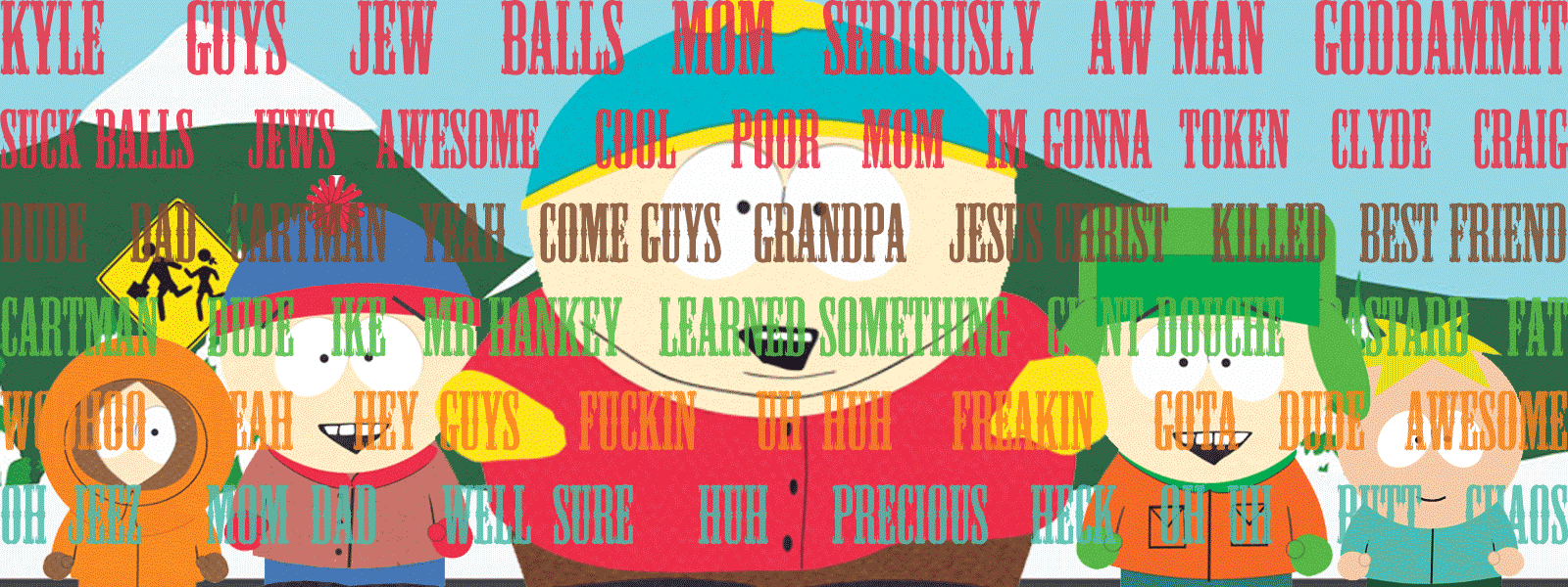
South Park follows four fourth grade boys (Stan, Kyle, Cartman and Kenny) and an extensive ensemble cast of recurring characters. This analysis reviews their speech to determine which words and phrases are distinct for each character. Since the series uses a lot of running gags, common phrases should be easy to find.
The programming language R and packages tm, RWeka and stringr were used to scrape South Park episode transcripts from the internet, attribute them to a certain character, break them into ngrams, calculate the log likelihood for each ngram/character pair, and rank them to create a list of most characteristic words/phrases for each character. The results were visualized using ggplot2, wordcloud and RColorBrewer. Full scripts on Github.
Method & Summary Statistics
Complete transcripts (70,000 lines amounting to 5.5 MB) were downloaded from BobAdamsEE’s github repository SouthParkData from the original source at the South Park Wikia page.
I used the stringr package to condense each speaker’s text into one large unformatted string. From there, I used the tm package to pre-process the text (to lowercase, remove punctuation, numbers and white space; remove stop words) and form a corpus, which contained more than 30,600 unique words spoken more than 836,000 times. Reducing the sparsity brought that down to about 3,100 unique words. Processing the text reduced it further to our final subset of roughly 1,000 unique words and phrases.
29 characters with the most words were retained, and the remaining 3,958 speakers combined into one “all others” category so as not to lose the text.
| speaker | words | speaker | words | speaker | words |
|---|---|---|---|---|---|
| cartman | 61110 | jimmy | 3738 | narrator | 1737 |
| stan | 34762 | gerald | 3285 | principal.victoria | 1732 |
| kyle | 31277 | jimbo | 3157 | jesus | 1714 |
| randy | 14994 | announcer | 2900 | mayor | 1603 |
| butters | 13690 | wendy | 2893 | craig | 1412 |
| mr..garrison | 9436 | sheila | 2794 | reporter | 1400 |
| chef | 5493 | liane | 2477 | satan | 1291 |
| mr..mackey | 4829 | stephen | 2245 | linda | 1285 |
| sharon | 4284 | kenny | 2112 | all.others | 152172 |
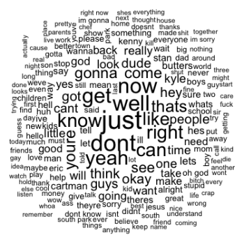
Exploring the text
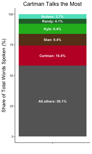
Overall (total words spoken by character / total words spoken), Cartman accounts for the biggest share of words.
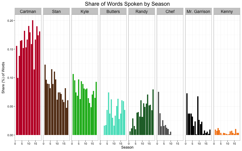
It's no surprise that Kenny accounts for a measly 1-2% per season or that Cartman accounts for 15-20% of words (overall, he accounts for 16.4%).
Butters and Randy have become more integral characters over time, leading to a stark increase in their share of words and decrease in Stan and Kyle's share. Chef's share declines over time and ultimately ends completely after his death in season 10. Mr. Garrison trails off after becoming Mrs. Garrison in season 9, returning in season 12's "Eek, a Penis!" episode.
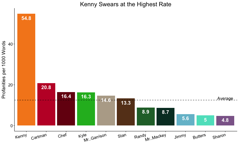
Profanity
Though Kenny doesn't speak as much as the rest of the characters, he swears at a much higher rate.
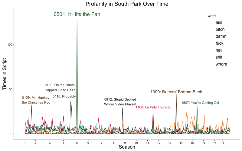
Individual swear words have been featured in different episodes: shit is common in "You're Getting Old" as well as the record-breaking episode "It Hits the Fan," while hell takes over in successive episodes "Do the Handicapped Go to Hell?" and "Probably." Ass and bitch share the spotlight in "Le Petit Tourette" and bitch shines in "Butters' Bottom Bitch." If you look closely, you can see a marked decreased in ass (red) and increase in fuck (orange). Cartman drove both words' usage, showing either a character development (growing up?) or a shift in preference by the writers.
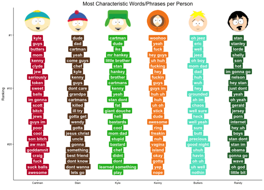
Identifying Characteristic Words using Log Likelihood
Each corpus was analyzed to determine the most characteristic words for each speaker. Frequent and characteristic words are not the same thing - otherwise words like “I”, “school”, and “you” would rise to the top instead of unique words and phrases like “professor chaos”, “hippies” and “you killed kenny.”
Log likelihood was used to measure the unique-ness of the ngrams by character. Log likelihood compares the occurrence of a word in a particular corpus (the body of a character’s speech) to its occurrence in another corpus (all of the remaining South Park text) to determine if it shows up more or less likely that expected. The returned value represents the likelihood that the corpora are from the same, larger corpus, like a t-test. The higher the score, the more unlikely.
The chi-square test, or goodness-of-fit test, can be used to compare the occurrence of a word across corpora.
$$\chi^{2} = \sum \frac{(O_i-E_i)^{2}}{E_i}$$
where O = observed frequency and E = expected frequency.
However, flaws have been identified: invalidity at low frequencies (Dunning, 1993) and over-emphasis of common words (Kilgariff, 1996). Dunning was able to show that the log-likelihood statistic was accurate even at low frequencies:
$$2\sum O_i * ln(\frac{O_i}{E_i})$$
Which can be computed from the contingency table below as $$(2 * ((a * log(\frac{a}{E1}) + (b * log(\frac{b}{E2})));$$
$$E1 = (a+c) * \frac{a + b}{N};
E2 = (b+d) * \frac{a + b}{N}$$
| Group | Corpus.One | Corpus.Two | Total |
|---|---|---|---|
| Word | a | b | a+b |
| Not Word | c | d | c+d |
| Total | a+c | b+d | N=a+b+c+d |
| Group | Cartmans.Text | Remaining.Text | Total |
|---|---|---|---|
| ‘hippies’ | 36 | 5 | 41 |
| Not ‘hippies’ | 28170 | 144058 | 172228 |
| Total | 28206 | 144063 | 172269 |
Computed:
E1 = 28206*(41/172269) = 6.71
E2 = 144063*(41/172269) = 34.28
LL = 2*(36log(36/6.71) + 5log(5/34.28)) = 101.7
Based on the overall ratio of the word “hippies” in the text, 41/172269 = 0.00023, we would expect to see hippies in Cartman’s speech 6.71 times and in the remaining text 34.28 times. The log likelihood value of 101.7 is significant far beyond even the 0.01% level, so we can reject the null hypothesis that Cartman and the remaining text are one and the same.
Only ngrams that passed a certain threshold were included in the log likelihood test; for unigrams, 50 occurrences, for bigrams, 25, for tri-grams, 15, 4-grams, 10 and 5-grams 5. Each ngram was then compared to all speakers, including those who said it 0 times (using 0.0001 in place of 0 to prevent breaking the log step of the formula). If the number of times the speaker said the word was less than expected, the log likelihood was multiplied by -1 to produce a negative result.
For this analysis, a significance level of 0.001 was chosen to balance the number of significant ngrams with significance. 1.31% of ngrams were found to be significantly characteristic of a given character.
| Level | Critical.Value | p.Value | Percent.Sig |
|---|---|---|---|
| 5% | 3.84 | 0.05 | 7.92 |
| 1% | 6.63 | 0.01 | 5.21 |
| 0.1% | 10.83 | 0.001 | 3.66 |
| 0.01% | 15.13 | 0.0001 | 2.83 |
The results were then filtered to include each word two times or less: once for the speaker most likely to say it (highest LL) and once for the speaker least likely to say it (lowest LL).
Ranking
Finally, the results were ranked using the formula
LL∗ngram.length
Ranking was used to condense the range of log likelihoods (-700 to 1000+). The ranking formula includes ngram length because longer ngrams appear fewer times in the text, leading to lower log likelihoods, but carry more semantic meaning.
References
Dunning, T. (1993) Accurate Methods for the Statistics of Surprise and Coincidence. Computational Linguistics, 19, 1, March 1993, pp. 61-74.
Kilgarriff. A. (1996) Why chi-square doesn’t work, and an improved LOB-Brown comparison. ALLC-ACH Conference, June 1996, Bergen, Norway.